#' % Averaging filters
#' % Wolfgang Scherr
#' % 10th February 2021
#' (c) Carinthia University of Applied Sciences
#' All rights reserved. For educational purposes only.
#' SystemC-AMS models created with [Coside](https://www.coseda-tech.com/coside-overview).
#+ echo=False
#-------------------------------------------------------------------
import shutil
import matplotlib
import matplotlib.pyplot as plt
import numpy as np
from numpy.fft import rfft # import Numpy/FFT
# see e.g.: https://stackoverflow.com/questions/27306474/plotting-fft-from-a-wav-file-using-python
def fft_plot(t,sig,xlabel,ylabel,title):
Fs = len(t) / max(t) # Sampling frequency
nfft = 2**np.floor(np.log2(len(t))) # Use next highest power of 2 greater
# than or equal to length(x) to calculate FFT.
fftx = rfft(sig,int(nfft)) # Take FFT, padding with zeros so that length(fftx) is equal to nfft
NumUniquePts = int(np.floor((nfft+1)/2.0)) # Calculate the number of unique points
fftx = fftx[0:NumUniquePts] # FFT is symmetric, throw away second half
mx = abs(fftx) / float(nfft) # Take the magnitude of FFT of x and
# scale the FFT so that it is not a function of the length of x
# multiply by two (see technical document for details)
# odd nfft excludes Nyquist point
if nfft % 2 > 0: # odd number of points FFT
mx[1:len(mx)] = mx[1:len(mx)] * 2
else: # even number of points FFT
mx[1:len(mx) -1] = mx[1:len(mx) - 1] * 2
f = np.arange(0, NumUniquePts, 1.0) * (Fs / nfft) # create frequency array
fig, ax = plt.subplots() # plot FFT
ax.plot(f, mx)
ax.set(xlabel=xlabel, ylabel=ylabel, title=title)
ax.grid()
plt.show()
#-------------------------------------------------------------------
#' # Moving average filters
#' This are filter structures, which calculates the average
#' of a defined amount of input samples continuously.
#' Which each new sample, the furthest 'away' sample is removed
#' again:
#+ echo=False, results = 'hidden'
#-------------------------------------------------------------------
shutil.copyfile('../averaging/doc/average_simple_schematic.svg','figures/average_simple_schematic.svg');
#-------------------------------------------------------------------
#' 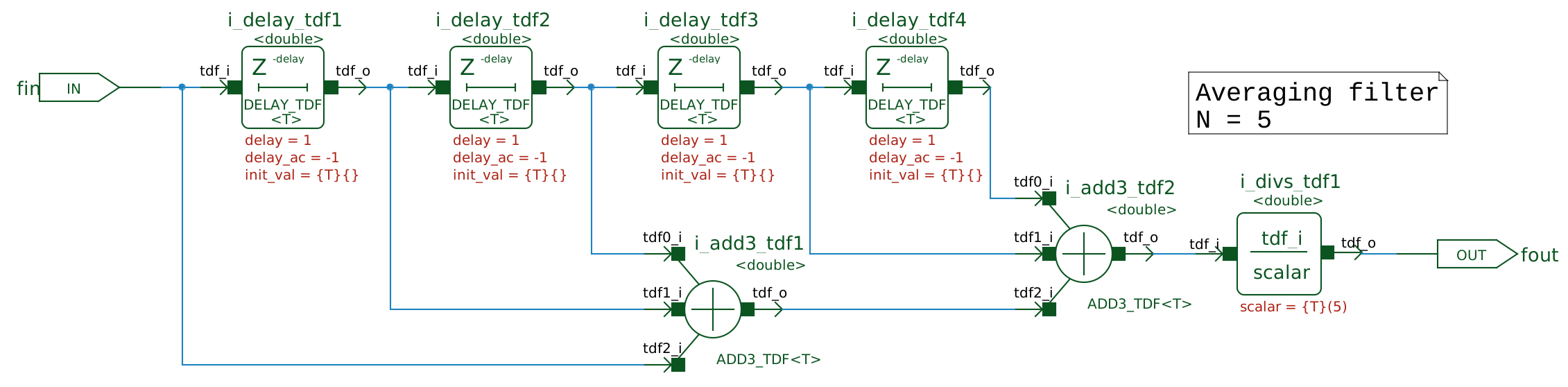 #' The difference equation for a 5-tap moving averaging filter is:
#' $y[n] = \frac{1}{5}(x[n] + x[n-1] + x[n-2] + x[n-3] + x[n-4])$
#' $x[n]$ is the actual sample, $x[n-1]$ is the last sample,
#' $x[n-2]$ is the next-to-last sample and so on.
#' The difference equation for a 5-tap moving averaging filter is:
#' $y[n] = \frac{1}{5}(x[n] + x[n-1] + x[n-2] + x[n-3] + x[n-4])$
#' $x[n]$ is the actual sample, $x[n-1]$ is the last sample,
#' $x[n-2]$ is the next-to-last sample and so on.
#' In a general form, the equation looks for a filter with length N like:
#' $y[n] = \frac{1}{N}\sum_{k=0}^{N-1}x[n-k]$
#' As this filter levels out fast changes, it has a
#' low-pass characteristics, let's check if this is true.
#' So we do the z-transform: $x[n-k]\rightarrow X[z]z^{-k}$ and get:
#' $Y[z] = \frac{1}{N}X[z]\sum_{k=0}^{N-1}z^{-k}$
#' Finally, we can write the transfer function as:
#' $H[z] = \frac{Y[z]}{X[z]} = \frac{1}{N}\sum_{k=0}^{N-1}z^{-k}$
#' Looking at the frequency behavior at the unit cycle $z = e^{j\omega}$
#' ([z transform](https://en.wikipedia.org/wiki/Z-transform)),
#' using $\sum_{k=0}^{n}r^k = \frac{1-r^{n+1}}{1-r}$
#' ([finite sum of the geometric series](https://en.wikipedia.org/wiki/Geometric_series))
#' and using $e^{j a} = cos(a) - j sin(a)$
#' ([Euler's formula](https://en.wikipedia.org/wiki/Euler%27s_formula)) we get:
#' $H[e^{j\omega}] = \frac{1}{N}\sum_{k=0}^{N-1}e^{-j\omega k} = \frac{1}{N}\frac{1-e^{-j\omega N}}{1-e^{-j\omega}}
#' = \frac{1}{N}\frac{e^{-\frac{j\omega N}{2}}\left(e^{\frac{j\omega N}{2}}-e^{-\frac{j\omega N}{2}}\right)}
#' {e^{-\frac{j\omega}{2}}\left(e^{\frac{j\omega}{2}}-e^{-\frac{j\omega}{2}}\right)}
#' = \frac{1}{N}\frac{sin \frac{\omega N}{2}}{sin \frac{\omega}{2}}e^{-\frac{j\omega}{2}(N-1)}$
#' # Frequency response plot for averaging filters
#' We plot the absolute transfer function for several length N from 0 to half the normalised sample frequency $f_s$.
#+ echo=False
#-------------------------------------------------------------------
# average lengths
Ns = [1,2,3,4,5,10]
# plot H(f), normalized 0 ... 0.5*fs
f = np.arange(0.0, 0.5, 0.001)
fp = f*np.pi
fig, ax = plt.subplots()
for N in Ns:
H = np.abs((np.sin(fp*N)+1e-99)/(N*np.sin(fp)+1e-99)) # 1e-99 avoids division by zero
# and correct gain at f=0
ax.plot(f, H, label='N='+str(N))
ax.set(xlabel='normalised sampling freqency [f/fs]', ylabel='attenuation',
title='simple averaging filter (different length N)')
ax.grid()
ax.legend()
# fig.savefig("average_filter.png")
plt.show()
#-------------------------------------------------------------------
#' # Check frequency response by simulation
#' We will use SystemC-AMS using the TDF MoC for transient noise and AC simulation.
#+ echo=False, results = 'hidden'
#-------------------------------------------------------------------
shutil.copyfile('../testbenches/doc/avg_simple_tb_schematic.svg','figures/avg_simple_tb_schematic.svg');
#-------------------------------------------------------------------
#' 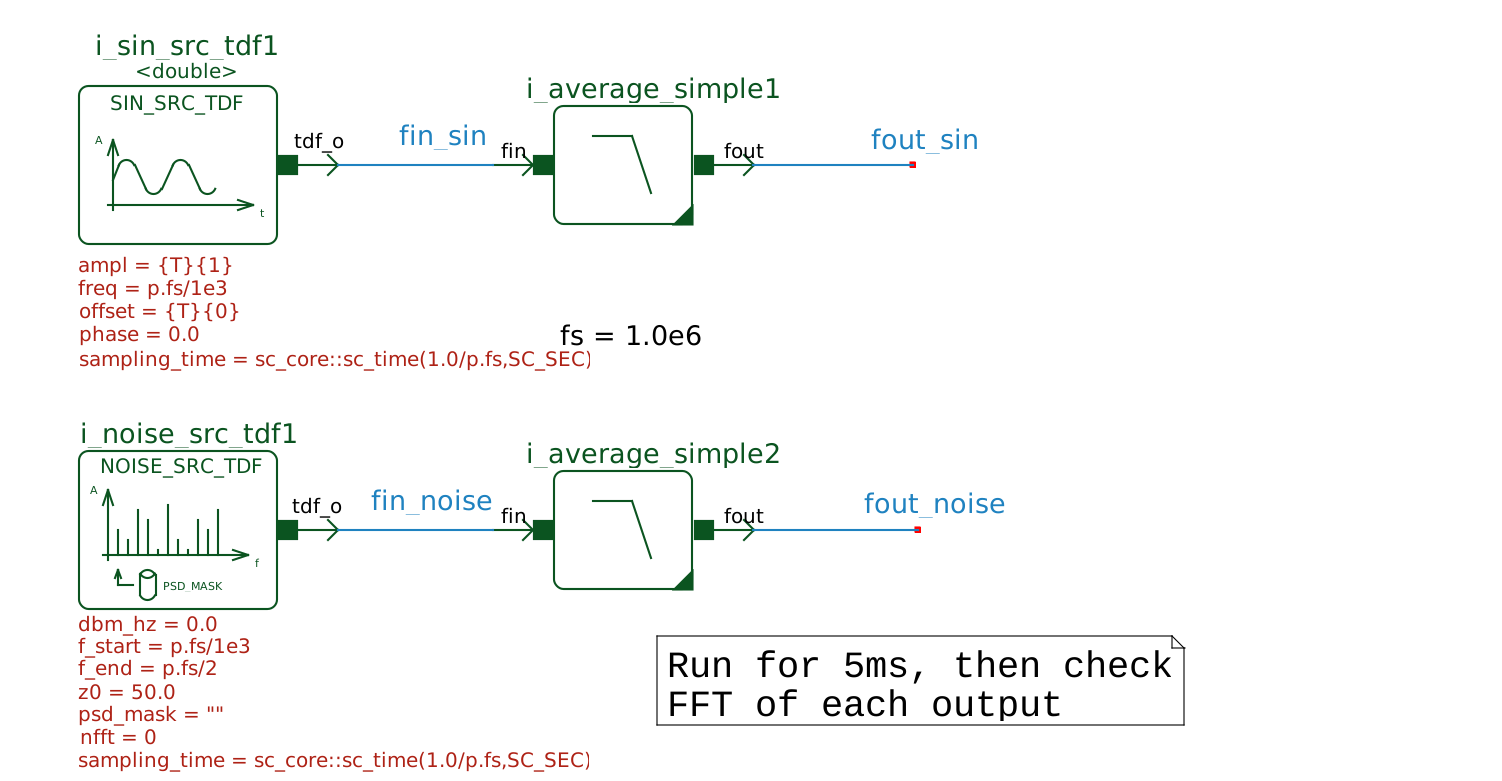 #' First, we send a noise signal into the filter (with constant power up to $f_s/2$):
#+ echo=False
#-------------------------------------------------------------------
dat = np.loadtxt('../DEBUG/testbenches/avg_simple_tb_tran.dat', comments='%', unpack=True)
t=dat[0]
fin=dat[1]
fft_plot(dat[0],dat[1],'input freqency [Hz]','input level','TRAN: simple averaging filter (N=5)')
#-------------------------------------------------------------------
#' Then we look at the FFT of the transient simulation result on its output:
#+ echo=False
#-------------------------------------------------------------------
fft_plot(dat[0],dat[2],'input freqency [Hz]','output level','TRAN: simple averaging filter (N=5)')
#-------------------------------------------------------------------
#' Finally, we do an AC simulation and look at the result (as absolute value):
#+ echo=False
#-------------------------------------------------------------------
dat = np.loadtxt('../DEBUG/testbenches/avg_simple_tb_ac.dat', comments='%', unpack=True)
f=dat[0]
fout_re=dat[3]
fout_im=dat[4]
fout_abs = np.sqrt(fout_re**2+fout_im**2) # calculate square-root of squared re+im parts
fig, ax = plt.subplots() # plot FFT
ax.plot(f, fout_abs)
ax.set(xlabel='input freqency [Hz]', ylabel='output attenuation',
title='AC: simple averaging filter (N=5)')
ax.grid()
plt.show()
#-------------------------------------------------------------------
#' # Area and power consumption (qualitative)
#' The requirement for such a simple moving average filter of length N,
#' assuming a single-bit input is:
#'
#' First, we send a noise signal into the filter (with constant power up to $f_s/2$):
#+ echo=False
#-------------------------------------------------------------------
dat = np.loadtxt('../DEBUG/testbenches/avg_simple_tb_tran.dat', comments='%', unpack=True)
t=dat[0]
fin=dat[1]
fft_plot(dat[0],dat[1],'input freqency [Hz]','input level','TRAN: simple averaging filter (N=5)')
#-------------------------------------------------------------------
#' Then we look at the FFT of the transient simulation result on its output:
#+ echo=False
#-------------------------------------------------------------------
fft_plot(dat[0],dat[2],'input freqency [Hz]','output level','TRAN: simple averaging filter (N=5)')
#-------------------------------------------------------------------
#' Finally, we do an AC simulation and look at the result (as absolute value):
#+ echo=False
#-------------------------------------------------------------------
dat = np.loadtxt('../DEBUG/testbenches/avg_simple_tb_ac.dat', comments='%', unpack=True)
f=dat[0]
fout_re=dat[3]
fout_im=dat[4]
fout_abs = np.sqrt(fout_re**2+fout_im**2) # calculate square-root of squared re+im parts
fig, ax = plt.subplots() # plot FFT
ax.plot(f, fout_abs)
ax.set(xlabel='input freqency [Hz]', ylabel='output attenuation',
title='AC: simple averaging filter (N=5)')
ax.grid()
plt.show()
#-------------------------------------------------------------------
#' # Area and power consumption (qualitative)
#' The requirement for such a simple moving average filter of length N,
#' assuming a single-bit input is:
#'
#' - Area: (N-1) flip-flops, (N-2) full adder
#' - Power: flip-flops (N-1) @ fs, full adder log2(N-2) @ fs
#'
#' For our example with N=5, 4 FF and 3 full adder are required.
#' For an averager with N=16, this goes up to 15 FF and 14 full adder.
#' The question is now, is this the best we can do?
#' # Improved implementation of averaging filters
#' The simple averaging filter delivers the moving average result with the same
#' rate as given by its input. But when using this filter for decimation, this is
#' not really needed. So by some translations we can show, that there is a more
#' efficient way to achieve the same result.
#' The intermediate steps lead to the very same behavior as the simple averager, we
#' spare the simulation for these ones here.
#' In the first step, we create an integrator where we add the actual and subtract the
#' Nth sample using a N-stage differentiator. The integrator needs only log2(N) FF and
#' log2(N) half adders. So not really better than before...
#+ echo=False, results = 'hidden'
#-------------------------------------------------------------------
shutil.copyfile('../averaging/doc/average_improved_schematic.svg','figures/average_improved_schematic.svg');
#-------------------------------------------------------------------
#' 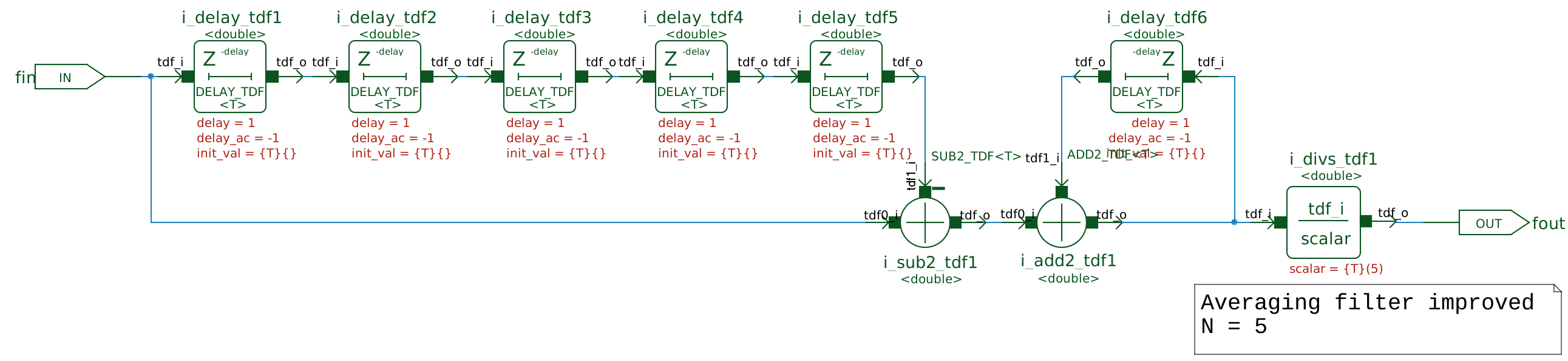 #' It seems that the next step does not really make sense, as it increases the bit width for the differentiator.
#' So it looks we made it even worse, but just wait a bit. It will get much better in a moment...
#+ echo=False, results = 'hidden'
#-------------------------------------------------------------------
shutil.copyfile('../averaging/doc/average_impr_rearr_schematic.svg','figures/average_impr_rearr_schematic.svg');
#-------------------------------------------------------------------
#'
#' It seems that the next step does not really make sense, as it increases the bit width for the differentiator.
#' So it looks we made it even worse, but just wait a bit. It will get much better in a moment...
#+ echo=False, results = 'hidden'
#-------------------------------------------------------------------
shutil.copyfile('../averaging/doc/average_impr_rearr_schematic.svg','figures/average_impr_rearr_schematic.svg');
#-------------------------------------------------------------------
#' 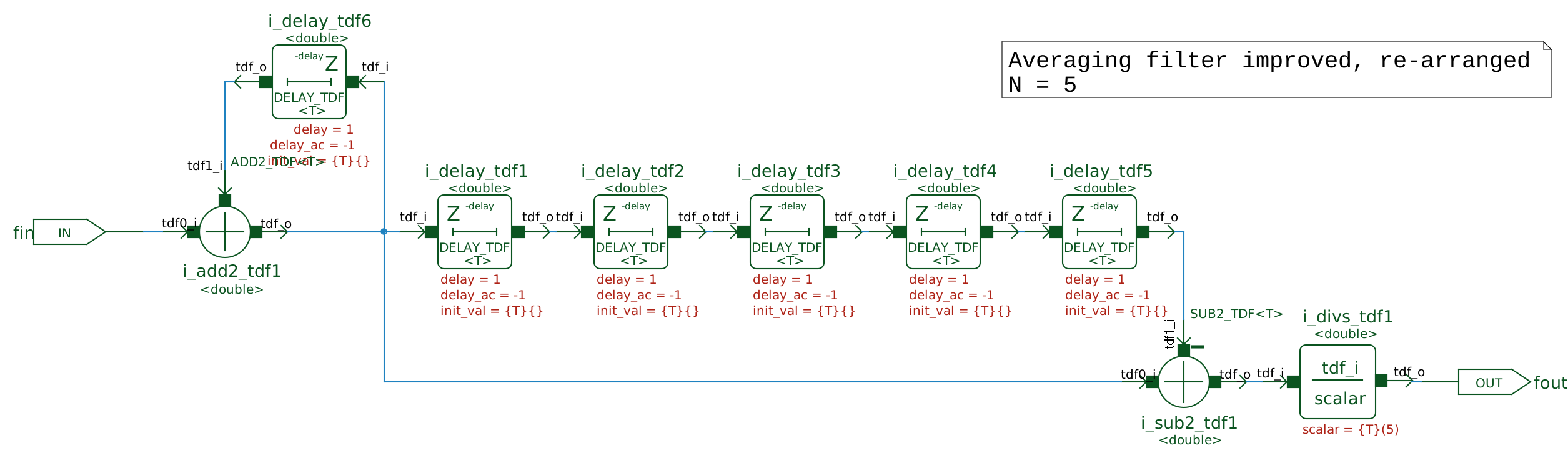 #' Now we introduce the decimation between these two stages. This means that the N-stage differentiator
#' can be reduced to a single stage running at the frequency of $f_s/N$:
#+ echo=False, results = 'hidden'
#-------------------------------------------------------------------
shutil.copyfile('../averaging/doc/hogenauer_cic_schematic.svg','figures/hogenauer_cic_schematic.svg');
#-------------------------------------------------------------------
#'
#' Now we introduce the decimation between these two stages. This means that the N-stage differentiator
#' can be reduced to a single stage running at the frequency of $f_s/N$:
#+ echo=False, results = 'hidden'
#-------------------------------------------------------------------
shutil.copyfile('../averaging/doc/hogenauer_cic_schematic.svg','figures/hogenauer_cic_schematic.svg');
#-------------------------------------------------------------------
#' 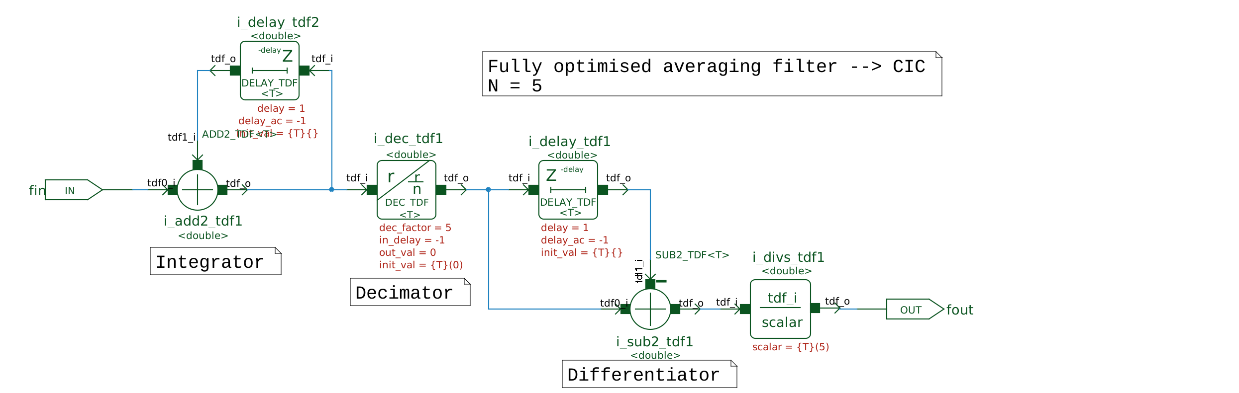 #' The requirement for such an average filter of length N, assuming a single-bit input is now:
#'
#' The requirement for such an average filter of length N, assuming a single-bit input is now:
#'
#' - Area: 2*log(N) flip-flops, log2(N) half adders, log2(N) full adders
#' - Power: flip-flops log(N) @ fs, log2(N) @ fs/N, half adder log2(N) @ fs, full adder log2(N) @ fs/N
#'
#' For our example with N=5: 6 FF, 3 half adder, 3 full adder are required.
#' For an averager with N=16: 8 FF, 4 half adder, 4 full adder is more efficient than the simple solution!
#' I spare the power estimation here, as I believe you see the advantage on that one by yourself.
#' This brings us to the Hogenauer filter, also called CIC filter, as described e.g.
#' [here by Matthew P. Donadio](http://dspguru.com/files/cic.pdf).
#' # Verify the new filter
#' We do again a transient simulation with a band-limited noise on the input to check the
#' frequency response.
#+ echo=False
#-------------------------------------------------------------------
dat = np.loadtxt('../DEBUG/testbenches/filter_tb_tran.dat', comments='%', unpack=True)
fft_plot(np.delete(dat[0],[0,1]),np.delete(dat[1],[0,1]),'input freqency [Hz]','input level',
'TRAN: CIC filter (N=5)')
#-------------------------------------------------------------------
#' When we look at the FFT of the transient simulation result on its output, we get 5 times
#' less samples on the output for the FFT.
#' The data we analyse is similar to an zero-order hold with 5*fs connected after the decimation.
#+ echo=False
#-------------------------------------------------------------------
fft_plot(np.delete(dat[0],[0,1]),np.delete(dat[5],[0,1]),'input freqency [Hz]','output level',
'TRAN: CIC filter (N=5)')
#-------------------------------------------------------------------
#' Be aware, the output spectrum basically 'ends' at a five times lower frequency, so to say.
#' Everything above the new fs/2 = 100kHz is folded back down into the signal band. Furthermore, all
#' notches at 200kHz and 400kHz of the upper sampling frequency fold back to 0 Hz on the lower
#' (output) sampling frequency.
#' It is better to see if we look at the decimated output data at fs=200kHz. here we can see the
#' original frequency response of the averaging filter within 0-500kHz folded into 0-100kHz.
#+ echo=False
#-------------------------------------------------------------------
dat = np.loadtxt('../DEBUG/testbenches/simple_tb_cic_decimated.dat', comments='%', unpack=True)
fft_plot(dat[0],dat[1],'output freqency [Hz]','output level','TRAN: CIC filter (N=5)')
#-------------------------------------------------------------------
#' It also demonstrates that a 1.O. averaging filter is not really good for decimation,
#' you should always consider higher order filters.
#' # Conclusion
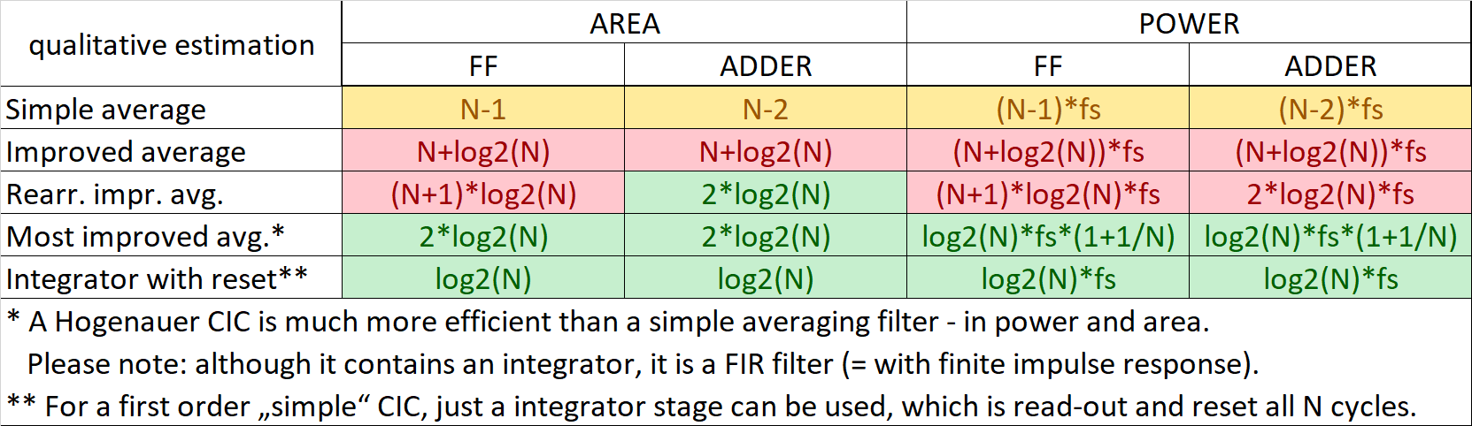
#' This report gave a quick introduction to averaging filters, from a very basic design to
#' broadly used CIC filters. The improvement in power consumption and area was briefly illustrated
#' as well in a qualitative sense.
#' Here the final result in a compact table:
#'  #' The report finally passes on to a nice paper explaining CIC filters in more depth.